Simulating Mixing Time with Computational Fluid Dynamics

The efficiency of mixing operations often has a big impact on production costs and product quality. The issue frequently boils down to designing an agitator that will provide the required level of mixing in as short a time as possible. The most common approach, building a scale model and performing physical experiments, introduces delays into the lead-time predictions. Computer simulation has been slow to take root in this area because of the difficulty of modeling the complex flow created by the impeller. Several recent approaches provide dramatic improvements in simulating flow in an agitated system. An investigation of the advantages and disadvantages of these new modeling options shows that the latest computational fluid dynamics (CFD) software provides excellent accuracy, well within the range of error of experimental methods.

Mixing time is usually the critical parameter in determining the efficiency of an agitated system. It is common to use correlations derived from experimental mixing time when designing an agitator. Correlations have many limitations, however. Usually the experiments are performed using a small-scale vessel, and the impeller geometry is not exactly the same as that used in the full-sized tank. Most correlations are based on measurements with single impellers, while multiple impeller systems are commonplace on production tanks. Another problem is that the feed location relative to impeller location may be different in the laboratory and large-scale systems. Because of these and other factors, significant inaccuracies are normally found in blend time predictions.

The Potential of CFD
CFD has long had the potential to improve the agitator design process by allowing engineers to simulate the performance of alternative designs on the computer, eliminating the guesswork in trying to match the tank and internals, the scale and the fluid properties. CFD involves the solution of the governing equations for fluid flow, heat transfer and chemistry in tens or hundreds of thousands of computational cells in the defined flow domain. The use of CFD enables engineers to obtain solutions for problems with complex geometry and boundary conditions. A CFD analysis yields values for species concentration, fluid velocity and temperature throughout the solution domain. A key advantage of CFD is that it provides the flexibility to readily change design parameters such as tank scale, flow regimes, impeller location, and number of impellers. It also provides a quick and easy route for determining mixing time.

Impeller Models
While CFD has become extremely popular for solving general flow problems in process industries, it has had somewhat less use in mixing applications. The primary reason is that the continual motion of the impeller, often in a baffled vessel, introduces complexity into the resulting flow field. During the past several years, a number of methods have been introduced to address this problem while keeping computational time at a reasonable level. The simplest approach, called the fixed velocity or velocity data method, models the impeller implicitly. Time-averaged velocity components and turbulence quantities are substituted for the actual impeller in the fluid cells of the CFD model. This steady-state formulation allows for the modeling of other time-dependent processes such as blending and free surface prediction. An important prerequisite of this method is the availability of reliable velocity and turbulence data, which is normally collected using laser Doppler velocimetry.

Explicit modeling of the impeller geometry is done through two methods without the need for experimental data as impeller boundary conditions. The first is called the multiple reference frames (MRF) model and is a steady-state approximation that simplifies the analysis by using multiple frames of reference. This method evolved from an earlier CFD practice in which the entire fluid flow problem was solved in a single frame of reference attached to the impeller. In this rotating frame, the impeller velocity would be zero and the tank wall would be assigned a rotational speed opposite that of the reference frame. Unfortunately, this rotating frame model is not valid for baffled tanks, where, in the frame of the impeller, the baffles would be moving through the oncoming fluid. This problem can be overcome by using separate or multiple reference frames for the baffles and the impeller. The impeller frame is a rotating one; the baffle frame is a stationary one. The solution proceeds with a steady transfer of information across a pre-defined interface between the two frames.

The other explicit model makes use of a sliding mesh. With this method, the tank is divided into two regions, as with the MRF model. One region, associated with the tank and baffles, remains stationary. The other region, associated with the impeller, rotates relative to the stationary mesh. The two grids slide past each other in a time-dependent manner, exchanging information at the cylindrical interface. The sliding mesh method is useful for examining start-up transients, or to accurately predict the periodic flow pattern in stirred reactors. The penalty is the calculation time, which can be an order of magnitude longer than that needed for steady state calculations.

Modeling the Turbulence
A number of turbulence models are available to model the turbulent hydrodynamics in a mixing tank. These include various Reynolds Averaged Navier-Stokes (RANS) models, in which the equations are time-averaged. The most common of these approaches are the k-e model and the Reynolds Stress model. Large eddy simulation (LES) is another technique of growing popularity, in which time averaging is applied to only the smallest turbulent eddies, i.e. those that are smaller than a typical cell size. Larger eddies are computed directly in this time-dependent model. Direct numerical simulation (DNS) of turbulent flow is done by computing the full range (all scales) of turbulent eddies. Because it requires a very fine computational grid and small time-step, it continues to be an impractical approach for large industrial applications. Despite the number of turbulence models available, no definitive studies investigating blend time have yet identified the best to be used for this purpose.

Substantial improvements have been made in CFD software in recent years that make it more practical than ever to combine these impeller and turbulence models for solving industrial problems. While older software versions limited explicit impeller models to relatively simple geometries, the newest software can model geometry of virtually any complexity. In addition, the sliding mesh model can be combined with the LES turbulence model to provide the ultimate in agitated system modeling accuracy. The comparatively high computational time required for this approach is less of a deterrent today than it would have been a few years ago because of the ongoing advances in computational power and speed.

Scope of the study
In this study the advantages and disadvantages of the various modeling options are investigated. Mixing times are determined based on the equilibrium concentration of a dispersed tracer. Three systems representing typical configurations were assessed: a flat bottomed vessel containing a single radial pumping impeller, a single axial pumping impeller, and a dual axial/radial impeller combination. The turbulent flow field in each tank configuration was calculated using RANS and LES turbulence models. The impellers are modeled using the sliding mesh model, the multiple –reference frames model and the velocity data method. The CFD mixing time estimates were compared to experimental measurements and to empirical correlations.

Mixing time calculations were performed by two different methods. The first used the unsteady tracking of a number of neutrally buoyant particles. After release, the turbulent dispersion of the particles was tracked, and particle concentration was sampled at various times.

The second method followed the transport of a tracer liquid, similar to a dye injection. The tracer was added near the liquid surface, and concentrations were monitored throughout the vessel as a function of time. This approach is similar to the most common experimental methods. It makes use of a key advantage of CFD - that multiple locations can be sampled simultaneously to show concentration changes in many locations in the tank.

The mixing time t99, is defined as the time taken for the uniformity, U, to reach 0.99, where

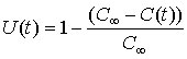
In this expression, C of infinity is the equilibrium concentration, and C(t) is the concentration at a point at some instant in time. The quantity t99 is determined at various locations in the tank and averaged to obtain the mixing time.

Accuracy within experimental error
Results of the study include predictions of velocity fields as well as blend times, and provide contrasts between the different impeller and turbulence models used. An evaluation of the turbulence models based on the velocity distribution in the tank showed the RSM turbulence model matched the experimental data far better than the k-e type models for both the pitched blade and Rushton turbines. That RSM provides the best flow field results suggests that it would offer the best overall predictions of blend time among the steady-state RANS turbulence models.

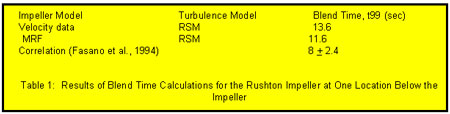
To explore the blend time predictions, several cases were examined. In one, the Rushton turbine blend time, t99, was computed for a single location below the impeller using both the velocity data model and the MRF model with a number of turbulence models. The blend times, some of which are summarized in Table 1, suggest that the Reynolds stress model yields good results for both the velocity data and MRF impeller models.

When the blend time calculations for the Rushton impeller and the RSM turbulence model were compared at another location in the tank, the MRF model returned a value of 10 sec while the velocity data model returned a value of 11.6 sec. That is, in both locations the velocity data model returned a slower blend time than the MRF model. This trend was also observed for the pitched blade turbine and the mixed impeller case.

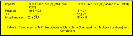
When blend times in four locations were sampled and the results averaged, the values were found to be within the correlation ranges suggested by Fasano et al (1994). These results are summarized in Table 2.

For the sliding mesh impeller model, two turbulence models were used: the Reynolds stress model and the LES model. While a transient calculation was not performed to obtain the full blending time, results in the early stages showed that the tracer begins to spread at about the same rate from the point of injection for both turbulence models. A qualitative comparison of the dispersion of the tracer suggests that the RSM model predicts a more uniform dispersion while the LES model predicts a more irregular pattern influenced by the instantaneous unsteady velocity field. More research into this area is planned.

The large-scale simulations described in this article can determine the elapsed time before complete blending occurs. With the exception of the LES model, they do not include the effects of mixing at the micro level. This work is currently being studied by several groups of researchers worldwide. Another development that can be expected in the near future is the ability to go beyond blending and model the chemical reactions that are normally the reason for agitating the mixture in the first place. This could be extremely useful for many applications such as those where competitive reactions take place and the type of mixing that occurs may favor one reaction over another. Modeling chemical reactions will increase the difficulty of the CFD simulation. This doesn't present any theoretical challenges but greatly increases the amount of computational resources required to solve the complete problem. Modeling reactions will also require a turbulence model such as LES that is capable of measuring instabilities that are averaged out in the RANS models. Several pioneering researchers have begun the process of conceptualizing this type of reaction but no commercial products have yet been released.

Reference:

Fasano, J.B., A. Bakker, and W.R. Penney, Advanced Impeller Geometry Boosts Liquid Agitation, Chemical Engineering, Aug. 1994.

In U.S., contact: Fluent Inc., 10 Cavendish Court, Centerra Resource Park, Lebanon, NH 03766. Ph: 603-643-2600, Fax: 603-643-3967. Visit Fluent's web site at http://www.fluent.com

Subscribe to our free e-mail newsletter.

Click for a free Buyer's Guide listing.