Compressible Flow Refresher

In production plants, there are many situations where pressure drops of process vapors and gases need to be calculated. Unlike liquids, gases are compressible, and the change in the conditions of the fluid as it moves down the pipe must be considered in these calculations. Because of this, quick refresher on the basic theoretical and empirical formulas required to calculate these pressure drops can help engineers solve day-to-day operating and design problems.

Many empirical formulas¹ and charts¹ have been used over the years to calculate the pressure drop of various gases flowing through pipes. The main constraint of these methods is that they usually may only be used to calculate pressure drops smaller than 10% of the absolute initial pressure of the fluid. This constraint is due to the fact that the properties of the fluid will change significantly as the pressure and temperature of the fluid changes due to flow. The advent of computer calculations eliminated this problem, allowing easy calculation of conditions throughout the entire range of subsonic flow.

Theoretical Analysis of Adiabatic Flow
Practical Use
No Need to Go Through all the Details
References

---

Theoretical Analysis of Adiabatic Flow (Back to Top)
Since most piping found in a typical production facility is fairly short, the system can best be analyzed theoretically by assuming it to be adiabatic. To begin this analysis, the first definition needed is that of Mach number, given by²:

Next, if a fluid is flowing in a pipe at a mach number, M, then the length of pipe required for the fluid to go from mach number M, to a mach number of 1 (speed of sound) is denoted by L_max and given by²:

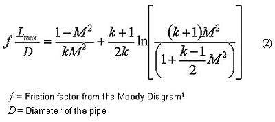
The maximum theoretical speed a subsonic fluid can reach is mach 1.

Now say that a gas is flowing in a pipe, starting at a velocity M₁ and ending at a velocity M₂. Using equation (2) it can be shown that the length of pipe required for the fluid in this system to go from velocity M₁ to M₂ is be given by²:

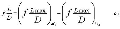
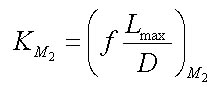
The subscript M₁ and M₂ and imply the use of equation (2) evaluated at those mach numbers. Of course in real world applications equation (3) is not much use because piping systems are never straight, but rather filled with valves, fittings, and instrumentation. To make equation (3) useful, a definition of the Resistance Coefficient¹ (K) is needed:

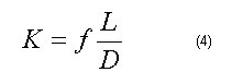
Using this definition equation (3) becomes:

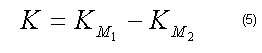
K is the overall resistance coefficient for the piping system being analyzed, and it is a function of the configuration of the piping and its components, the properties of the fluid, and the velocity of the fluid. There are a number of ways to calculate these resistance coefficient values³.

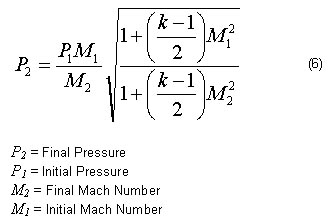
All that is now needed to calculate the pressure drop of any subsonic compressible flow application is a way to relate the initial fluid pressure to the final fluid pressure using only the initial and final mach numbers and the physical constants of the fluid. This is easily given by the equation²:

Practical Use (Back to Top)
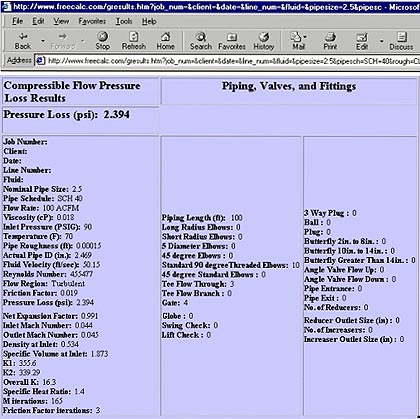
Now let's use these methods to solve a real-life problem. Look at a typical air system with 100 ACFM of air flowing through a 2 ½" line at 90 PSIG and 70 F. The air in the line must travel through 100 ft of line containing 10 elbows, 4 gate valves, and 3 tees to get to its destination. What is the pressure drop through this section of line?

First, the initial Mach number in found using equation (1), the properties of the air (k=1.4), the initial pressure of the air, and the system pipe size. Remember that the density of the air at 90 PSIG can be found by the ideal gas law, and the velocity can be found from the flow rate, density, and pipe size. Using equation (1) this gives M₁ = 0.044.

Next the resistance coefficient must be found for this system. In this case, resistance coefficient correlations from Crane¹ where used. To use these correlations the friction factor, f, for this system must be found. This friction factor can be found from the Moody diagram¹ or the Colebrook Equation.

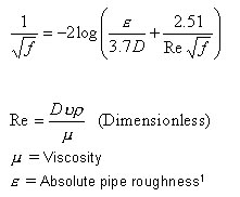
This equation shows that the friction factor depends on the properties of the fluid, its velocity, and the pipe size. Here it is evaluated here at the inlet conditions of the system. This is of minimal error because gas flow is usually very turbulent and the friction factor changes very slightly under these conditions. The friction factor at these inlet conditions is 0.019.

Using the resistance coefficient correlations from Crane, the piping configuration, and this friction factor, the overall resistance coefficient is found to be K = 16.3.

Using equation (2) and remembering that:

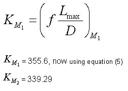
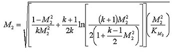
Now outlet or final Mach number, M₂ can be found using equation (2), and re-arranging it to get:

Remember:

Iteration yields M₂. In this example M₂ = 0.045.

With the outlet mach number M₂ now known, simple calculation of equation (6) can be done to determine the outlet or final pressure in the pipe, P₂. In this example P₂ is 102.306 PSIA, giving a pressure drop in the line of 2.394 PSI.

No Need to Go Through all the Details (Back to Top)
Although more complicated than calculating pressure losses for incompressible flows, use of the above equations makes compressible flow calculations possible throughout the operating ranges seen in most facilities. There is of course software available that can easily allow you to make these calculations without going through all the mathematics shown above. Unfortunately, many operations and design personnel may not have the time or resources to take advantage of these, or their use of a calculation of this type is not frequent enough to warrant the purchase and learning curve associated with one of these programs. To solve this problem, the author has produced an interactive web site that allows users to calculate the pressure drop of almost any subsonic compressible flow situation using only your browser. This application "On-line Compressible Flow Pressure Loss" and other helpful engineering calculations can be accessed for free at the author's web site at http://www.freecalc.com/.

Screen shot of John Kossik's pressure drop calculator.

References (Back to Top)

1. "Flow of Fluids Through Valves, Fittings, and Pipe", Technical Paper No. 410, Crane Co., 1985.
   
2. Shapio A.H., "Dynamics and Thermodynamics of Compressible Fluid Flow", Ronald Press, 1953.
   
3. Darby, R., "Correlate Pressure Drops through Fittings" Chem. Eng., pp.101-104, July 1999.

For more information: John Kossik, Beacon Engineers, 18940 Northeast 150th St., Woodinville, WA 98072. Tel: 425-742-9693. Fax: 425-883-2171.

John Kossik is a process engineer for Beacon Engineers Inc. (Seattle, WA).